How to make a publication-quality protein figure
From a default ribbon diagram to a 300 dpi PNG

Matic Broz, PhD16 min
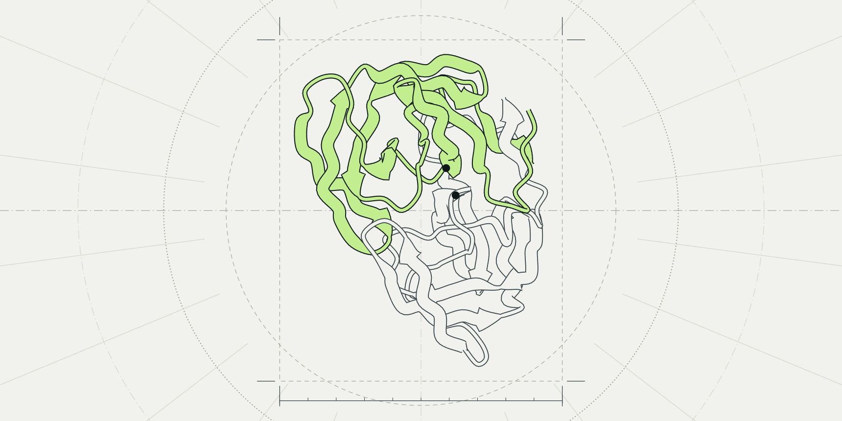
HIV-1 protease (PDB entry 1HSG) opens in the PDB viewer as a two-colour ribbon with 127 crystal waters floating around it and an inhibitor too small to read. It is a fine working view and a poor figure.
To turn it into one, hide the waters, show one style, colour by one property, light it with the Ray traced option and save the image from Export at the width the journal prints: 1,051 pixels for an 89 mm column at 300 dpi.
PyMOL gets there with ray and png figure.png, 10cm, dpi=300, ray=1.[3] This guide builds the figure in the PDB viewer by ProteinIQ, which draws with the Mol* engine and runs in the browser with no install,[9] and gives the PyMOL command beside each step.

Start from one structure and a clear view
A figure makes one point, so remove what does not serve it. For 1HSG that means the waters, and for most structures it means any chain that is not in the story.
- Open the PDB viewer, type
1HSGinto the search box and pressEnter. - In the panel beside the canvas, click the eye icon on the
HOHrow to hide the waters. - Drag to rotate, scroll to zoom, and stop when the feature you want to show faces you.
Reset the view, at the bottom right of the canvas, undoes a bad turn.
Rotate before you style. A view that hides the active site behind a loop cannot be fixed by colour. In PyMOL, fetch 1hsg downloads the entry as mmCIF by default, remove solvent deletes the waters and orient lines the structure up with the screen axes.[3]
Choose cartoon, surface or sticks
The three styles answer different questions, and a figure usually needs one of them for the whole protein and a second only for the part under discussion. A ribbon diagram or protein cartoon, the same thing under two names, shows how the chain folds. A surface shows what a ligand or partner can touch. Sticks show atoms and bonds, which only matter for a few residues.
| Style | Shows | Use it for | Avoid it when |
|---|---|---|---|
| Cartoon | Backbone path, helices as coils and strands as arrows | Fold, topology, domain layout, overall comparisons | The point is a specific atom contact |
| Surface | The outline a solvent probe can reach | Pockets, interfaces, electrostatic or hydrophobic patches | Secondary structure matters, because the surface hides it |
| Sticks | Every heavy atom and bond of the chosen residues | A ligand, a mutated residue, a catalytic triad | More than a few dozen residues, where they become clutter |
Representation menu; the PyMOL commands are show cartoon, show surface and show sticks.[3]In the viewer, point at Representation, the top button of the toolbar on the left of the canvas, and check Cartoon, Surface or Sticks. With nothing selected the menu acts on the whole structure; with something selected, its title changes to the selection and a style is added to it only. That is how you get a cartoon protein with one ligand in sticks.
Colour by chain, secondary structure, B-factor, pLDDT or hydrophobicity
Colour should carry one message that the caption can state in a sentence. Open Color in the toolbar and pick a scheme: Chain, Secondary structure, Element, B-factor, pLDDT or Hydrophobicity. As with styles, a selection limits the colour to itself.
| Colouring | Answers | Watch for |
|---|---|---|
| Chain | Which subunit is which | Two similar hues merge in greyscale print |
| Secondary structure | Where the helices and strands are | Says little about an all-strand protein such as 1HSG |
| B-factor | How mobile or disordered atoms were in the crystal | The scale is relative to one entry, so give the range and compare only within a structure |
| pLDDT | How confident a prediction is, residue by residue | Meaningful only for predicted models; crystal structures keep B-factors in the same column |
| Hydrophobicity | Where greasy and polar patches sit | Which scale is used, and the red to green default |
util.cbc colours by chain, spectrum b by B-factor and color red, ss h a secondary structure type.[3][6]B-factor
B-factor colours each atom by its temperature factor, so flexible loops stand apart from the rigid core. The number depends on the refinement program and the entry, so a loop that is red in one structure is not comparable with a red loop in another. State the range in the caption. In PyMOL, spectrum b, blue_white_red does the same, and minimum= and maximum= fix the range.[3]
pLDDT
A predicted model stores its confidence where a crystal structure stores B-factors, and pLDDT reads that column and colours by the usual pLDDT bands: above 90 very high, 70 to 90 confident, 50 to 70 low and below 50 very low.
To get a model to colour, search for a UniProt accession in the viewer, or predict one with AlphaFold 2 or ESMFold.
Hydrophobicity
The viewer has two hydrophobicity colourings, and they use different scales. Color, then Hydrophobicity, uses the Wimley and White scale for residues at membrane interfaces.[8] Under By attribute in the same menu, the Kyte-Doolittle entry colours by Kyte and Doolittle's hydropathy index. Name the scale in the caption either way.
The Hydrophobicity colouring runs from red to green by default. Cell Press asks authors not to put red and green together in a figure, so for a figure that goes to a journal choose a palette in By attribute that runs blue, white, red instead.[2] PyMOL has no built-in command for hydrophobicity; the PyMOL Wiki hosts a color_h script that uses the Eisenberg scale.[7]
Highlight a ligand and its contacts
The usual figure is a protein in pale cartoon with the ligand in sticks and its contacts marked. 1HSG holds the inhibitor indinavir, listed as MK1.
- Click
MK1in theLigandslist. The viewer selects it and zooms in. - Open
Colorand chooseElement. The menu title names the selection, so only the ligand changes. - Click
Clearabove the selection so later steps act on everything again. - Click
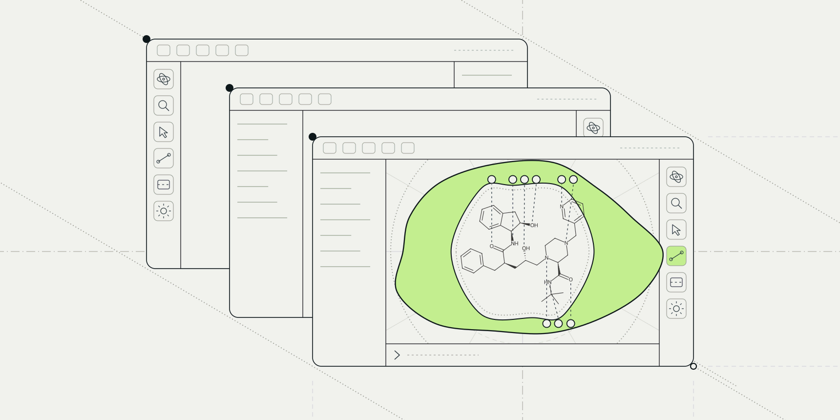
Ligand interactions, the first button of the second toolbar group. WithShow contacts in 3Don, dashed lines join the ligand to the residues it touches and the residues are labelled.
The panel lists each contact with its type and distance in ångströms, so the figure and the table agree. If the labels overlap, hide the kinds of contact you are not discussing with the coloured switches above the table. For the chemistry of what the dashes mean, see protein-ligand interactions.
In PyMOL, show sticks, resn MK1 draws the ligand and distance hbonds, resn MK1, polymer, 3.5, mode=2 draws polar contacts, where mode=2 shows only polar contact distances.[3]
Light the scene and set the background
Lighting, in the toolbar, has four settings: Flat, Outline, Soft shadows and Ray traced. Flat is standard lighting. Outline draws flat colour with black outlines, like an illustration. Soft shadows darkens crevices. Ray traced bounces light between surfaces and casts soft shadows.
The canvas looks grainy while you turn the structure and sharpens within a second or two once you stop. The exported image traces for longer than the canvas does, so it is cleaner than what you see. The option appears only when your graphics card supports it in the browser; on older or integrated graphics, Soft shadows is the closest look.
In PyMOL, ray renders the current view with its own ray tracer, which can take several minutes for a complex scene.[3] set ray_trace_mode, 1 adds black outlines.[5]
Background is a choice in the export dialog, covered next. Pick White for a journal. Pick Transparent for slides and posters, so the slide colour shows through behind the protein.
Export the image at the journal's size
Open Export, the download button at the bottom of the left toolbar, and stay on the Image tab. Size offers 1×, 2× and 4× the canvas, or Custom for a width and height in pixels. The line under it shows the result, for example 2408 × 2044 px at 2× in a 1,600 px wide browser window.
Background is Transparent, White or Black. Download PNG renders the image in the lighting you chose, and Copy puts it on the clipboard.
Journals ask for a width in millimetres and a resolution in dots per inch, so convert before you pick a size. The number of pixels is the width in millimetres divided by 25.4, times 300:
| Journal | Column | Width | Pixels at 300 dpi |
|---|---|---|---|
| Nature | Single | 89 mm | 1,051 |
| Nature | One and a half | 120 to 136 mm | 1,417 to 1,606 |
| Nature | Double | 183 mm | 2,161 |
| Cell Press | Single | 8.5 cm | 1,004 |
| Cell Press | One and a half | 11.4 cm | 1,346 |
| Cell Press | Full width | 17.4 cm | 2,055 |
Nature wants photographic images at a minimum of 300 dpi at the largest size they will be used, and says that raising the resolution in an art program does not improve quality.[1] Cell Press asks for at least 300 dpi for colour figures at the desired print size.[2] A rendered protein is not a photograph, but the safe reading is the same: export at the pixel width in the table or larger, and never enlarge a small export afterwards.
To export at an exact size, choose Custom and type the width in pixels. The height follows from what you type, so check it against the journal's depth limit. A size beyond what your graphics card can render is reduced, and the dialog marks it.
The command line takes the same request in PyMOL's syntax. png figure.png, 10cm, dpi=300 saves an image 10 cm wide at 300 dpi, which is 1,181 pixels, and a missing height keeps the canvas's proportions.[3]
The file format depends on the journal. Cell Press lists TIFF, PDF, EPS, JPG, PSD and PNG for production files.[2] Nature prefers TIFF or layered PSD for raster images and accepts high-resolution JPEG, but does not list PNG.[1] Export a white background first, then convert with Python and Pillow:
from PIL import Image

Image.open("figure.png").convert("RGB").save(
    "figure.tif", dpi=(300, 300), compression="tiff_lzw"
)
Nature recommends RGB and Cell Press asks for it when colour is used, and the conversion keeps RGB.[1][2] It also drops the transparency channel, which is why the white background matters.
The same figure in PyMOL
PyMOL separates drawing from saving: ray renders the view with the ray tracer and png writes it. Giving png the option ray=1 runs the ray trace first, at the size you ask for.[3] The commands below build the same figure as the steps above.
The viewer's Command line, at the bottom of the canvas, accepts PyMOL syntax, so you can try them there. It reads png the same way, but its ray turns on Ray traced lighting, and the ray=1 option of png is accepted without changing anything, because every export is rendered off screen.
| Step | In the viewer | In PyMOL |
|---|---|---|
| Open the entry | Search for 1HSG | fetch 1hsg |
| Remove the waters | Hide the HOH row | remove solvent |
| Cartoon, surface, sticks | Representation | show cartoon, show surface, show sticks, resn MK1 |
| Colour by chain | Color, Chain | util.cbc |
| Colour by B-factor | Color, B-factor | spectrum b, blue_white_red |
| Secondary structure | Color, Secondary structure | color red, ss h and color yellow, ss s |
| White background | Export, Background, White | bg_color white |
| Transparent background | Export, Background, Transparent | set ray_opaque_background, off |
| Ray-traced lighting | Lighting, Ray traced | ray |
| Save at 10 cm and 300 dpi | Export, Image, Custom | png figure.png, 10cm, dpi=300, ray=1 |
A complete PyMOL session for the opening figure reads:
fetch 1hsg
remove solvent
orient
show cartoon, polymer
util.cbc
show sticks, resn MK1
bg_color white
png figure.png, 10cm, dpi=300, ray=1
PyMOL's reference gives unset opaque_background followed by ray as the route to a transparent background, and the PyMOL Wiki describes the same switch as ray_opaque_background, which when off treats the background as an alpha channel.[3][4] The reference adds that PNG is the only image format PyMOL writes, so the TIFF step above applies there too.[3]
Common mistakes
| Problem | What you see | Fix |
|---|---|---|
| Screenshot of the window instead of an export | Toolbar and panel in the figure, pixelated at print size | Use Export, Image; it renders the canvas alone at the size you choose |
| Pixel width too small for the column | A blurred figure once the layout program scales it to 89 mm | Use the pixel widths in Table 3 or larger |
| Transparent PNG sent to a journal | An unexpected background after the file is flattened | Export with a white background |
| pLDDT colours on a crystal structure | Meaningless blues and oranges taken from B-factors | Use B-factor for crystal structures and pLDDT for predictions only |
| Red and green used together | A figure that readers with red-green colour blindness cannot parse | Choose a blue, white, red palette |
| No scale or range in the caption | A B-factor or hydrophobicity figure no one can read quantitatively | Give the attribute, scale and range in the caption |
After the figure
A still figure is one view. To show a structure from several sides in a talk, make a protein animation from the same scene. To hold it in your hand, 3D print the protein from the viewer's STL export. The PyMOL commands cheat sheet lists the rest of the syntax the viewer's command line understands, and the pLDDT guide helps you decide which parts of a prediction deserve a bright colour.
If the entry is the starting point rather than a file, how to open a PDB file covers every route in. For a flat contact diagram that a journal can print in black and white, PLIP draws protein-ligand interactions from the same structure.
Frequently asked questions
What resolution do journals want for protein figures?
Nature wants at least 300 dpi at the largest size a photographic image will be used, and Cell Press wants at least 300 dpi for colour figures at the desired print size.[1][2] At 300 dpi an 89 mm column is 1,051 pixels wide.
How do I make a transparent PNG of a protein?
In the PDB viewer, set Background to Transparent on the Image tab of Export and click Download PNG. In PyMOL, turn off ray_opaque_background and ray trace.[4]
What is the difference between ray and png in PyMOL?
ray renders the current view with PyMOL's ray tracer. png writes the image to disk, and its ray=1 option runs the ray trace first at the size given.[3]
How do I colour a protein by B-factor?
In the PDB viewer, open Color and choose B-factor. In PyMOL, run spectrum b, blue_white_red.[3]
Should I use cartoon, surface or sticks?
Cartoon for the fold, surface for what a partner can touch and sticks for the few residues under discussion. Most figures combine a cartoon for the protein with sticks for one ligand.