Analyze protein backbone phi/psi angles and classify favored, allowed, and outlier residues. Learn more
Input
Upload PDB or mmCIF coordinates, or enter a PDB ID. Analysis is free and runs in your browser.
What is a Ramachandran plot?
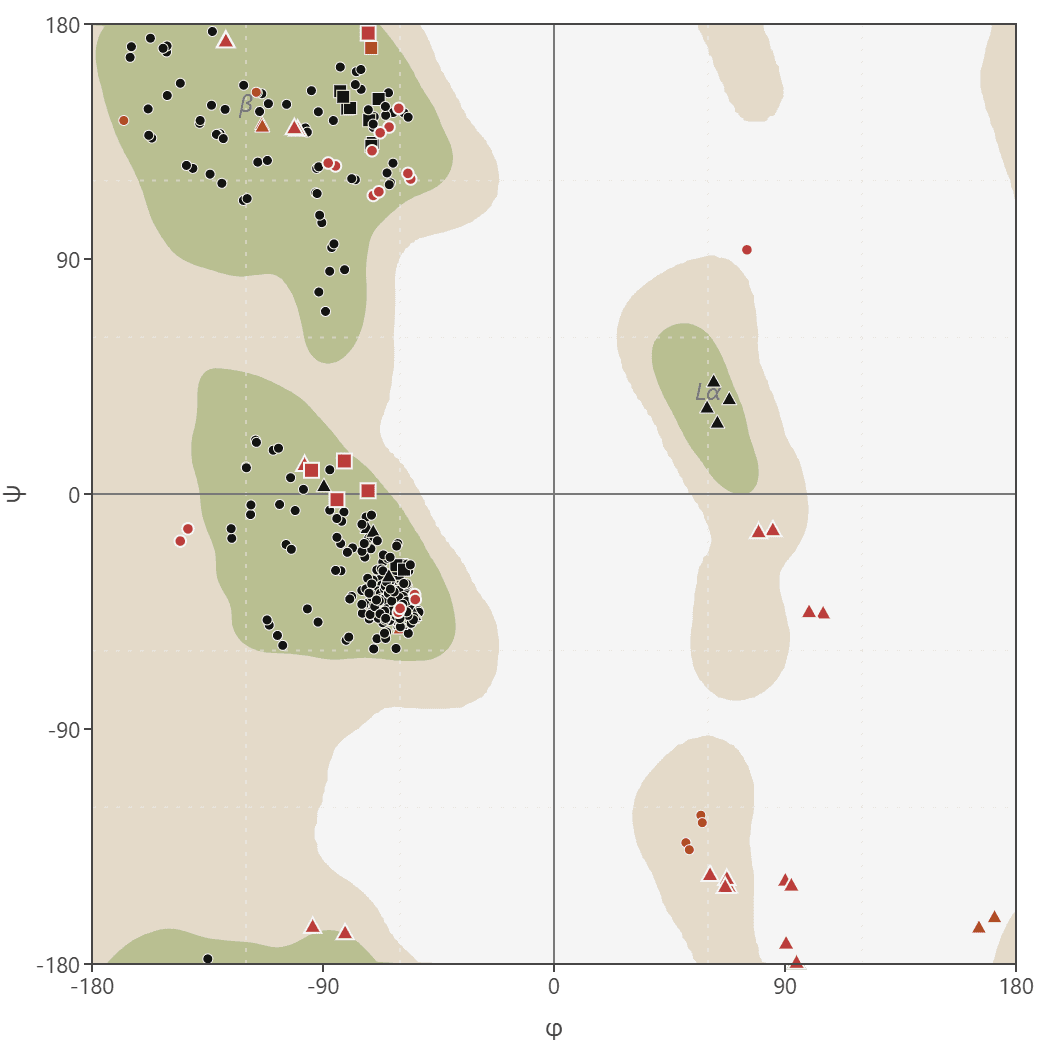
A Ramachandran plot is a two-dimensional visualization that maps the energetically allowed and forbidden backbone dihedral angles (φ and ψ) of the amino acid residues in a protein structure. Biochemists and structural biologists use it to study protein folding and to validate protein models. G.N. Ramachandran, C. Ramakrishnan, and V. Sasisekharan introduced it in 1963 in the Journal of Molecular Biology.
Most φ/ψ combinations force backbone atoms to clash, so they never occur in real structures. The combinations that remain form the allowed regions of the plot, which correspond to the common secondary structures: alpha helices, beta sheets, and turns.
Ramachandran analysis is a standard validation step for structures from X-ray crystallography and cryo-EM. A well-refined high-resolution structure places more than 98% of its residues in favored regions. Residues that fall outside the allowed regions, called outliers, usually point to a modeling error or a genuine strained conformation that has a functional reason.
How does a Ramachandran plot work?
Backbone dihedral angles
The protein backbone has three dihedral angles per residue. The phi (φ) angle is the rotation around the bond between the nitrogen and the α-carbon. The psi (ψ) angle is the rotation around the bond between the α-carbon and the carbonyl carbon. The omega (ω) angle at the peptide bond stays near 180° because of its partial double-bond character.
The φ angle is measured from four atoms: C(i-1), N(i), Cα(i), and C(i). The ψ angle uses N(i), Cα(i), C(i), and N(i+1). Because each angle depends on a neighboring residue, the first and last residue of every chain are missing one angle and do not appear on the plot.
Steric constraints
Ramachandran's original analysis modeled atoms as hard spheres with van der Waals radii and sampled every φ/ψ combination. Many combinations are forbidden because the atoms would clash, a constraint called steric hindrance, leaving a small set of allowed ranges that map directly onto secondary structure. Each allowed region sits in a characteristic part of the plot.
| Conformation | Approximate φ | Approximate ψ | Plot location |
|---|---|---|---|
| Beta sheet | -120° | +120° | Top left |
| Right-handed alpha helix | -60° | -45° | Bottom left |
| Left-handed alpha helix | +60° | +45° | Top right |
Residue-specific regions
The allowed regions differ by residue type because of side-chain geometry. The tool classifies and plots each residue against the reference set for its own class.
| Class | Allowed region behavior |
|---|---|
| General | The standard distribution shared by most amino acids, with φ predominantly negative |
| Glycine | A single hydrogen side chain gives minimal steric hindrance, so the allowed region is large and nearly symmetric |
| Cis-proline | Proline following a cis peptide bond has its own compact reference distribution |
| Trans-proline | A cyclic side chain locks φ near -60°, confining it to a narrow strip |
| Pre-proline | Residues immediately before a proline shift due to contact with the proline ring |
| Isoleucine or valine | β-branched side chains produce a distinct distribution from the general class |
Region classification
The tool uses the six residue classes and favored/allowed thresholds from the cctbx rama8000 validation tables. Classification uses reference masks sampled on a 2° grid. Near classification thresholds, results can differ from cctbx, which interpolates between reference values. The smoothed contours are a visual guide to those masks; points close to an edge should be interpreted using their reported classification. Proline uses the cis-like reference for −90° < ω < 90° and the trans-like reference otherwise, including twisted peptide bonds.
| Region | Population in well-refined structures | Meaning |
|---|---|---|
| Favored | ~98% of residues | Optimal backbone geometry |
| Allowed | ~2% of residues | Sterically possible but less common |
| Outlier | Remaining residues | Possible modeling error or a real strained conformation |
Input requirements
The tool reads PDB and mmCIF files with atomic coordinates. A scored residue needs N, Cα, and C, plus the preceding residue’s C and the following residue’s N. Proline also needs the preceding Cα to determine its reference class. Coincident or collinear atoms that make a dihedral undefined are excluded. Residues are connected using peptide-bond geometry rather than requiring consecutive author residue numbers. Use Enter PDB ID beside the upload control to fetch its mmCIF structure directly from the RCSB Protein Data Bank, or upload your own file. For multi-model files such as NMR ensembles, only the first model is analyzed. Load the 1HNR example to try the tool immediately; it contains the deposited backbone coordinates needed for this analysis.
Understanding the results
Plot interpretation
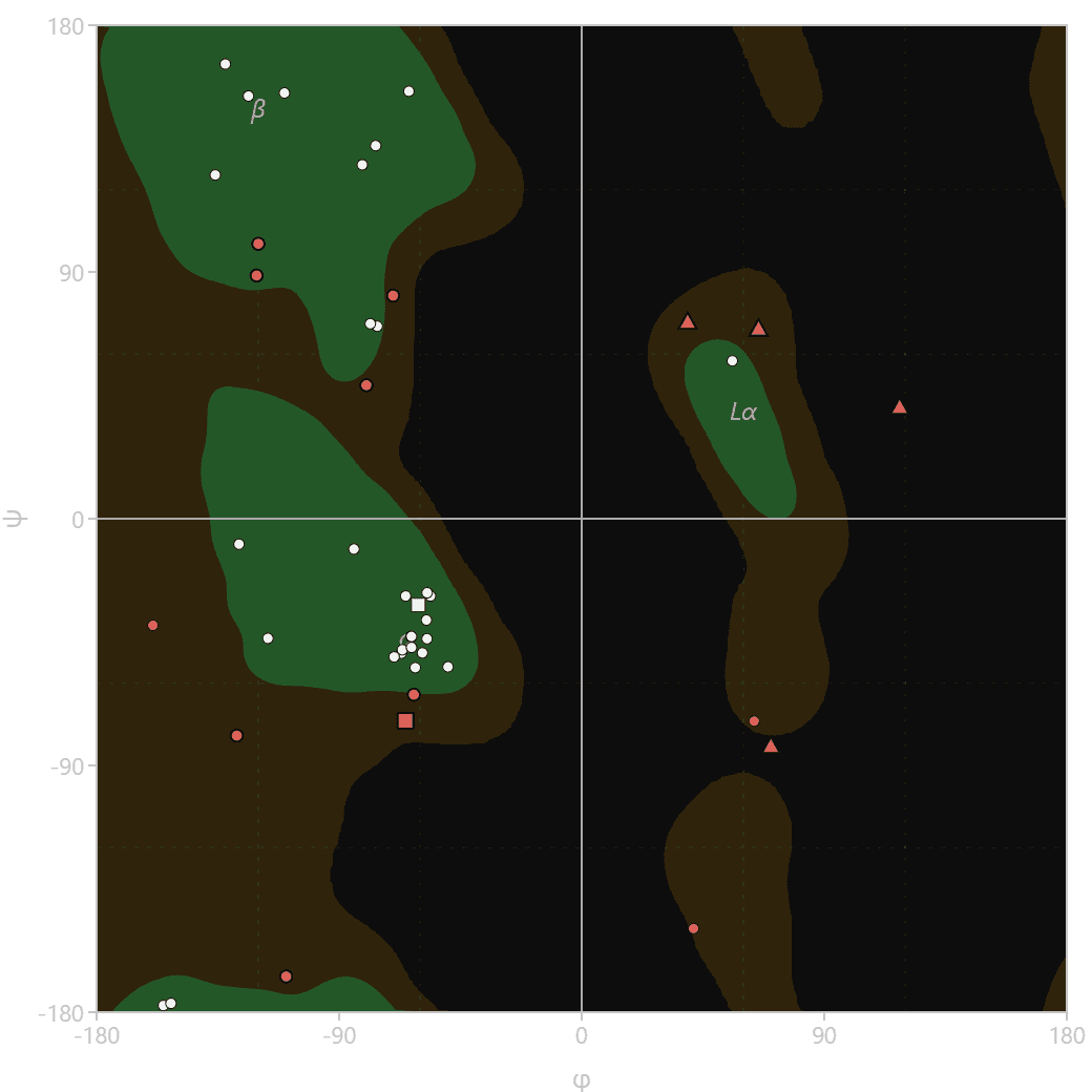
The plot opens on the General residue class, with only that class’s points and reference regions. Each class has its own distribution; glycine, cis-proline, trans-proline, pre-proline, and isoleucine/valine can be selected individually. Favored and allowed areas are shown for one class at a time, and outliers are red crosses.
All residues (overview) shows every scored residue without a reference background or secondary-structure labels. Each point retains its own class-specific classification. There is no single shared favored region for all six residue classes; use the class selector to compare points with their appropriate contours.
The view selector switches the plot to a single residue class and isolates that class's favored and allowed regions. Hover a point for a preview, or click or tap it to pin its name, number, chain, angles, residue class, and region in the residue inspector. Focus the plot and use Left/Right arrow keys to inspect residues, Home/End to jump to the first/last residue, and Escape to clear selection. Display options filter by chain, toggle the reference regions and annotations, hide outliers, and adjust point size.
Statistics panel
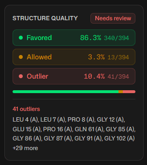
The summary reports counts and percentages for the residues currently shown on the plot and is named for the selected residue class. Choose All residues (overview) in the residue-class selector to see all classes together; clear chain filters and turn off Outliers only to see whole-structure totals. The overview has no reference areas; choose General or another individual class to restore its reference areas. The whole-structure backbone assessment retains its full denominator. Export Current selection (CSV) for the visible points or All residues (CSV) for all scored residues; the data table tab also retains all scored residues.
| Favored residues | Interpretation |
|---|---|
| Above 98% | Expected for high-quality structures |
| 95% to 98% | Acceptable for most purposes |
| Below 95% | May indicate structural problems that need investigation |
Outlier analysis
Use Outliers only to isolate flagged residues. Expand Inspect outliers and select a row to highlight its point and inspect its angles. All matching outliers are listed, and the data table tab lists every residue with its exact angles for sorting or export. Not every outlier is an error. Functionally important residues sometimes adopt strained conformations for catalysis or binding, so compare outlier positions with functional annotations before treating them as mistakes.
Analysis coverage
A note below the plot summary lists residues excluded from scoring, with their identifiers and reasons. Chain ends, missing atoms, chain breaks, undefined dihedrals, and proline residues without a usable ω angle are excluded from the percentage denominator. Coverage counts include residues with at least one parsed backbone atom in the first model; they do not count residues absent from the coordinate file.
Common applications
| Application | Purpose |
|---|---|
| Model validation | Assess crystal structures, NMR ensembles, and homology models |
| Structure refinement | Find residues that need manual adjustment during model building |
| Comparative analysis | Compare conformational states or mutants of the same protein |
| Teaching | Show how backbone geometry relates to secondary structure |
Cost
Ramachandran plot generation is free and runs entirely in your browser. No credits required.
Sources
- Ramachandran GN, Ramakrishnan C, Sasisekharan V. "Stereochemistry of polypeptide chain configurations." Journal of Molecular Biology 7, 95-99 (1963). doi:10.1016/S0022-2836(63)80023-6
- Lovell SC, et al. "Structure validation by Cα geometry: φ,ψ and Cβ deviation." Proteins 50, 437-450 (2003). doi:10.1002/prot.10286
- Williams CJ, et al. "MolProbity: More and better reference data for improved all-atom structure validation." Protein Science 27, 293-315 (2018). doi:10.1002/pro.3330
Related tools
MolProbity
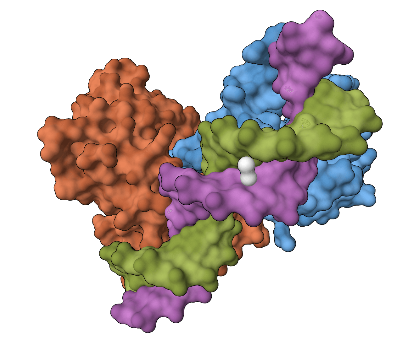
Validate protein structure quality with all-atom contact analysis, Ramachandran plots, rotamer assessment, and geometry checks.
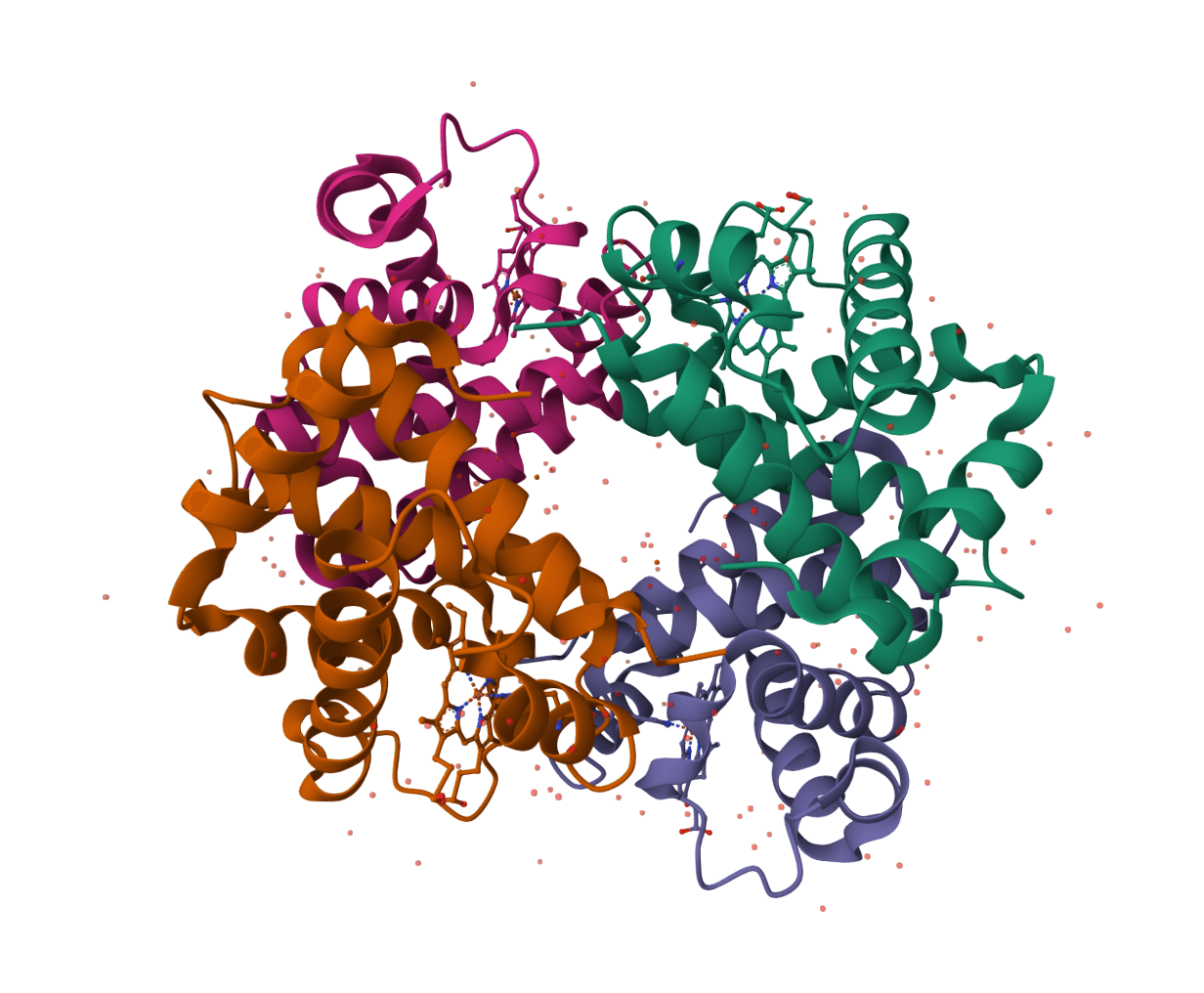
PDBsum
Generate a downloadable PDBsum structural summary report archive for a single protein structure.
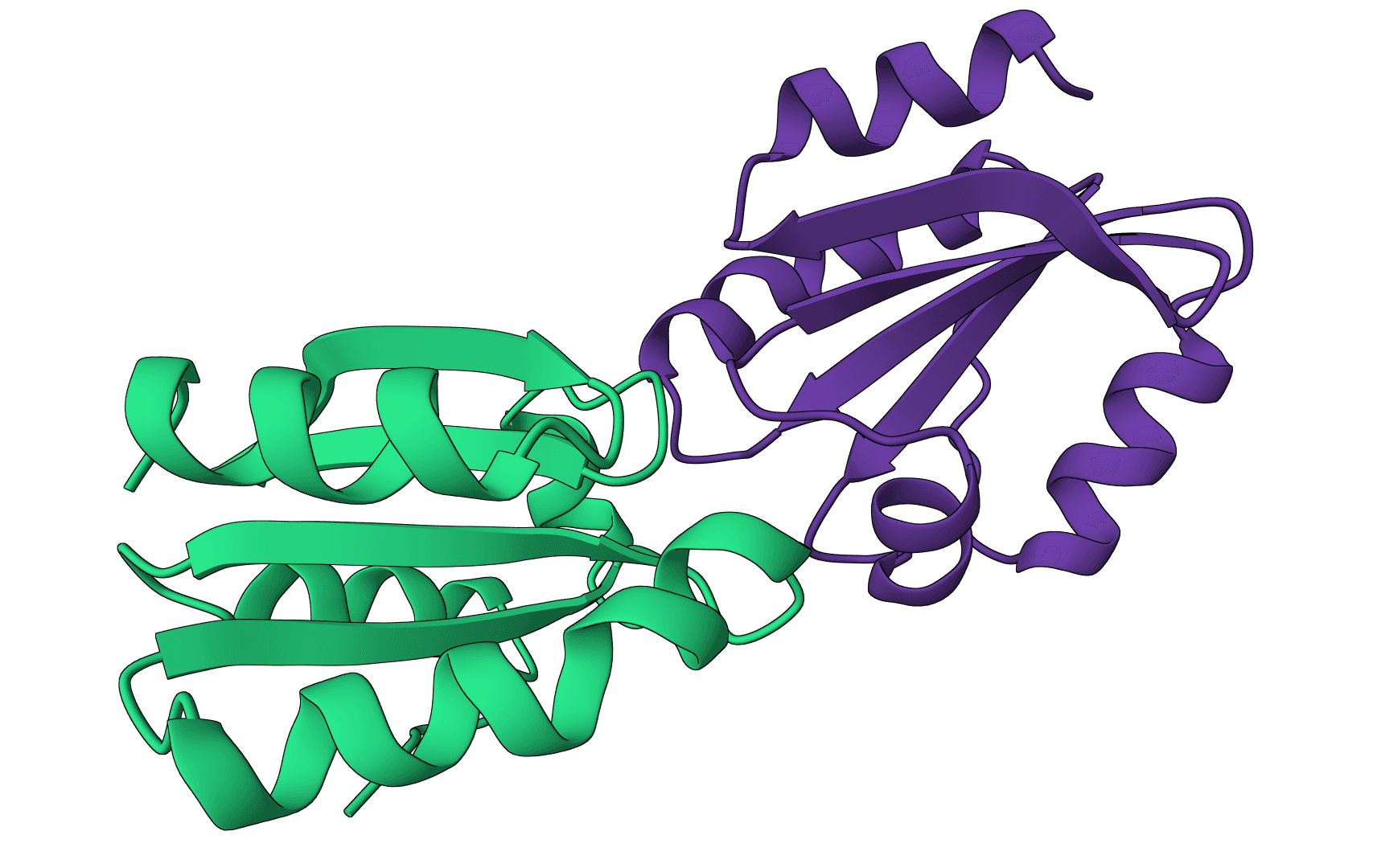
DockQ
Assess docking model quality by comparing predicted complexes against native references. DockQ v2.1.3 supports protein, nucleic-acid, and supported small-molecule interfaces with native metrics.
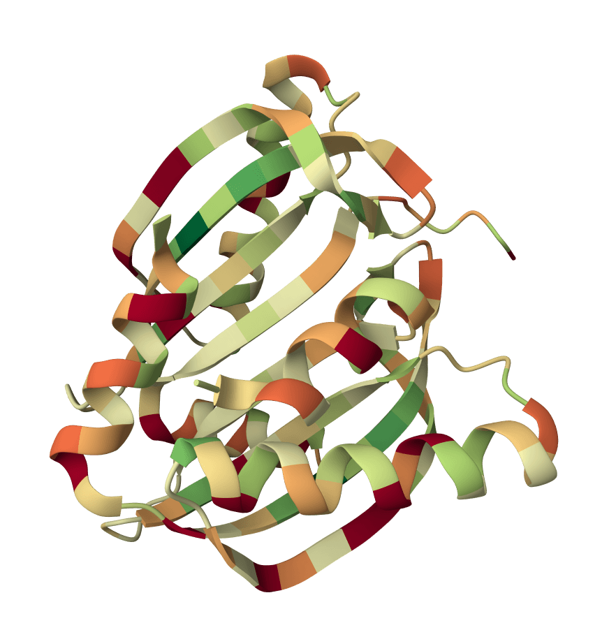
IPSAE
Scoring function for interprotein interactions in AlphaFold2, AlphaFold3 and Boltz predictions. Calculates ipSAE, ipTM, pDockQ, pDockQ2, and LIS scores to assess protein-protein interface quality.
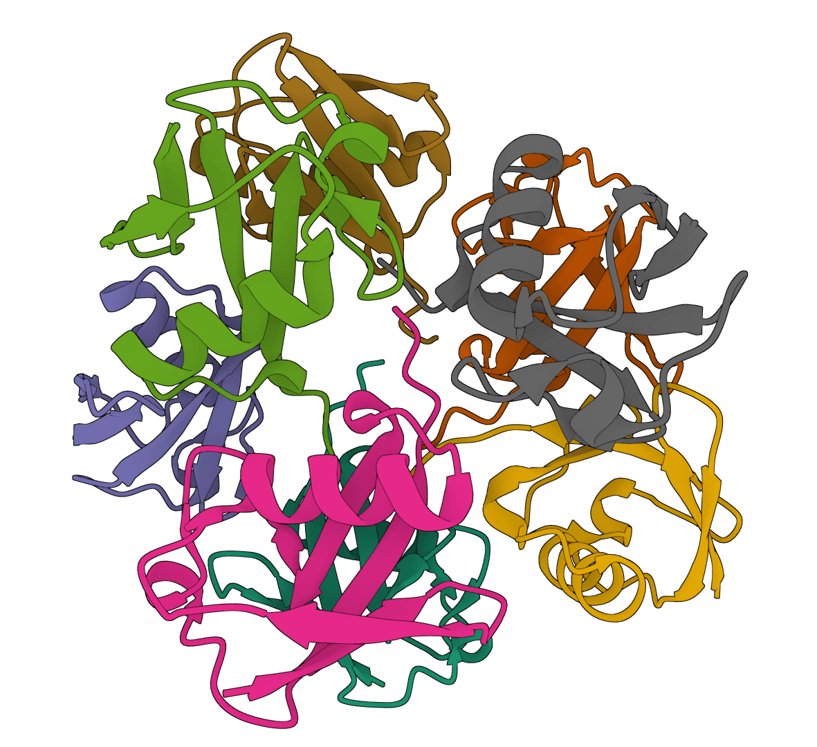
PoseBusters
PoseBusters validates generated or docked molecular poses with chemically and structurally grounded quality checks for molecular geometry, intermolecular interactions, and optional reference-pose agreement.
Protein charge plot
Plot net charge vs pH for protein sequences. Visualize how protein charge changes across pH 0-14 and identify the isoelectric point (pI) where the net charge crosses zero.
Hydropathy plot
Generate Kyte-Doolittle hydropathy plots to visualize hydrophobic and hydrophilic regions along protein sequences. Identify transmembrane domains and surface-exposed regions.
Hydrophobicity plot
Generate hydrophobicity plots using 24 different amino acid scales. Visualize hydrophobic and hydrophilic regions for protein analysis, epitope prediction, and membrane protein studies.
Protein scale profiler
Generate amino acid property profiles using 42 different scales spanning hydrophobicity, secondary structure propensity, flexibility, polarity, surface accessibility, antigenicity, and more.
DSSP
Assign protein secondary structure with the source DSSP program and return annotated mmCIF, legacy DSSP, residue geometry, hydrogen-bond statistics, and native files.