Related tools
AutoDock-GPU
GPU-accelerated molecular docking using the AutoDock4 force field. Up to 56x faster than serial AutoDock via CUDA parallelization of the Lamarckian Genetic Algorithm.
AutoDock Vina
AutoDock Vina is a widely-used molecular docking tool that predicts protein-ligand binding modes using physics-based force fields. Fast, reliable, and the gold standard for structure-based drug discovery.

PandaDock
Open-source molecular docking platform using physics-based scoring functions. CPU-optimized algorithms achieve sub-angstrom accuracy (0.014A RMSD) without GPU requirements.
SMINA
SMINA is a fork of AutoDock Vina with enhanced scoring functions, custom scoring support, and 10-20x faster minimization. Ideal for scoring function development, pose refinement, and high-performance docking workflows.
SurfDock
SurfDock is a surface-informed diffusion generative model for protein-ligand docking, published in Nature Methods 2024. It leverages protein surface geometry to guide a diffusion process for reliable and accurate protein-ligand complex prediction.
DiffDock-L
DiffDock-L is a state-of-the-art molecular docking tool that uses diffusion models to predict how small molecule ligands bind to protein targets. It generates multiple binding poses with confidence scores.
DynamicBind
DynamicBind is an AI-powered protein-ligand binding prediction tool that recovers ligand-induced conformational changes from unbound protein structures. It predicts both ligand binding poses and protein conformational changes.
SigmaDock
SigmaDock is a fragment-based molecular docking tool using SE(3) equivariant diffusion models to predict how small molecule ligands bind to protein targets. Presented at ICLR 2026, it generates multiple binding poses with Vinardo scoring.
DFMDock
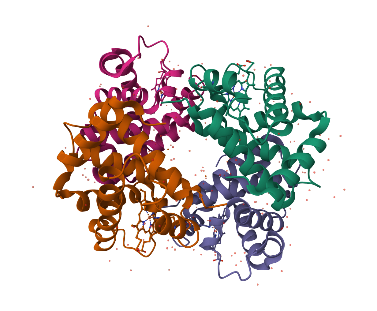
DFMDock (Denoising Force Matching Dock) is a diffusion model that unifies sampling and ranking for protein-protein docking within a single framework. It predicts docked poses for protein-protein complexes from unbound structures using denoising score matching with optional clash force guidance.
EquiDock
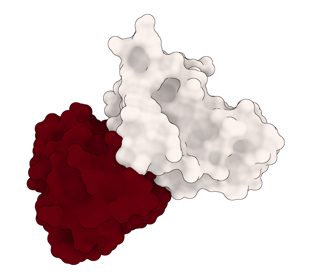
EquiDock is an SE(3)-equivariant graph neural network for rigid protein-protein docking. It predicts a binding pose for a protein-protein complex from unbound structures using geometric deep learning, with DIPS and DB5 pretrained checkpoints from the upstream release.
What is GNINA?
GNINA (pronounced "guh-NINA") is a molecular docking tool that combines traditional AutoDock Vina-style physics-based docking with deep learning CNN scoring functions. It achieves 73% pose prediction accuracy compared to Vina's 58% on redocking benchmarks, while maintaining practical computation times.
The hybrid approach uses Vina's search algorithm to explore binding poses, then applies convolutional neural networks to score and rank results. This gives you the reliability of physics-based sampling with the pattern recognition capabilities of deep learning.
For comprehensive virtual screening workflows, consider combining GNINA with ADMET-AI for pharmacokinetic predictions or Lipinski's Rule of Five for drug-likeness assessment.
How does GNINA work?
GNINA uses a two-stage docking pipeline that leverages both classical optimization and modern deep learning.
Stage 1: Pose sampling
The docking engine inherits Vina's Iterated Local Search algorithm with BFGS quasi-Newton optimization. It explores the binding space through random mutations of ligand position, orientation, and torsion angles, generating diverse candidate poses.
Stage 2: CNN scoring
Each candidate pose passes through an ensemble of convolutional neural networks trained to recognize protein-ligand binding patterns. The CNNs operate on 3D grids of Gaussian atom-type densities, learning spatial features that distinguish native binding modes from decoys.
The networks are trained on two objectives simultaneously:
- Pose classification: Predicting whether a pose is within 2Å RMSD of the experimental structure
- Affinity prediction: Estimating binding free energy in kcal/mol
CNN architectures
GNINA 1.3 includes models trained on the CrossDocked2020 v1.3 dataset:
Default ensemble uses five independent CNN models and averages their predictions. This provides the most robust scoring at the cost of increased computation.
Dense architecture uses twelve convolutional layers organized into three densely connected blocks. Each layer connects to all subsequent layers, improving gradient flow and feature reuse.
Knowledge-distilled models compress ensemble performance into a single faster model, making high-throughput screening more practical without significant accuracy loss.
Input requirements
Protein
GNINA accepts PDB files or RCSB PDB IDs. The protein should be prepared with hydrogens added and missing residues resolved. Use PDB Fixer for automated preparation if your structure has issues.
Ligand
You can provide ligands as SMILES strings, SDF files, or MOL2 files. The current ProteinIQ GNINA wrapper is intended for small-molecule ligands and automatically prepares 3D coordinates for SMILES inputs. Peptide-scale and macrocycle-scale ligands are not supported in this wrapper mode because they require more careful search-space and ligand-preparation control than this interface exposes.
Docking parameters
Exhaustiveness
Controls search thoroughness by setting the number of independent Monte Carlo runs. Higher values explore more of the binding landscape but increase computation time linearly. Values of 8-16 work well for most targets.
Number of poses
Specifies how many binding poses to return. GNINA uses RMSD-based filtering to ensure structural diversity, removing poses that are too similar to each other.
CNN model
Default ensemble averages predictions from multiple independently trained models. We recommend this for production use when accuracy matters more than speed.
Dense and Dense v1.3 use single deep CNNs with densely connected layers. Choose these when you need faster turnaround for large screening campaigns.
Knowledge-distilled (KD) models compress ensemble performance into a single faster model. Dense v1.3 KD and CrossDock 2018 KD provide near-ensemble accuracy at single-model speed, making them ideal for high-throughput screening.
CrossDock 2018 and General 2018 are models trained on the original CrossDocked dataset. They remain available for reproducibility with earlier work.
Redock 2018 is trained specifically on redocking tasks (predicting poses for ligands with known crystal structures).
CNN scoring mode
Controls how the CNN scoring function is applied during docking.
Rescore (default) runs the Vina search algorithm first, then re-scores the final poses with the CNN. This is the fastest mode and sufficient for most use cases.
Refinement uses the CNN during pose optimization, allowing the search algorithm to follow the CNN gradient toward better poses. This produces higher-quality poses but is approximately 10x slower than rescore mode. Use this when maximum pose accuracy matters for a single compound.
None disables CNN scoring entirely and uses only the Vina scoring function. This is equivalent to running standard AutoDock Vina and is useful when you only need physics-based scores.
Pose sort order
Controls how output poses are ranked.
CNN Score (default) ranks by the pose confidence score — how likely each pose is to be close to the true binding mode. This is the recommended ranking for most workflows.
CNN Affinity ranks by predicted binding strength (pKd). Use this when comparing binding affinities across poses matters more than pose quality.
Vina Energy ranks by the physics-based binding energy (kcal/mol). Use this for direct comparison with AutoDock Vina or Smina results.
Search box padding
Extra space added to the search box. Larger padding allows broader exploration but increases the search space and runtime.
Reference ligand autoboxing
By default, GNINA computes the search box from the entire protein structure, which can create a very large search volume for big proteins. If you know the approximate binding site, you can provide a reference ligand (e.g., a co-crystallized ligand from the same or a similar crystal structure) to focus the search.
Enable "Use reference ligand for search box" and paste the PDB or SDF content of a ligand already positioned in the binding site. GNINA will compute the docking box around this reference ligand, significantly improving both speed and result quality for large proteins.
Understanding the results
CNN score
The CNN pose score indicates confidence that a predicted pose is close to the true binding mode. Scores closer to 1.0 indicate higher confidence, while scores near 0 suggest the pose may be incorrect. GNINA ranks poses primarily by this score.
The CNN is trained to classify poses as "good" (within 2Å RMSD of the crystal structure) or "bad". The output probability directly reflects this binary classification confidence.
CNN Affinity (pKd)
Predicted binding affinity from the CNN head, reported in pKd units. Higher values indicate stronger predicted binding (e.g., pKd 8 ≈ nanomolar affinity, pKd 6 ≈ micromolar). This score is useful for ranking and comparing compounds but should not be interpreted as a precise thermodynamic measurement.
Vina Score (kcal/mol)
Traditional physics-based binding energy from the AutoDock Vina scoring function, reported in kcal/mol. More negative values indicate stronger predicted binding:
| Range | Interpretation |
|---|---|
| -4 to -6 | Weak binding |
| -6 to -8 | Moderate binding |
| -8 to -10 | Strong binding |
| < -10 | Very strong binding |
This score reflects the minimized Vina energy after CNN-guided pose optimization. It complements the CNN affinity by providing a physics-based energy estimate.
Interpreting results
Examine the top 3-5 ranked poses rather than relying solely on the highest-ranked prediction. Alternative binding modes within the top results may represent valid conformations. Visual inspection in PDB Viewer helps verify that predicted poses make chemical sense.
Comparison to other docking tools
| Feature | GNINA | AutoDock Vina | Smina | DiffDock |
|---|---|---|---|---|
| Method | Vina + CNN scoring | Physics-based + ML | Vina fork | Diffusion model |
| Pose accuracy | ~73% top-1 | ~58% top-1 | ~60% top-1 | ~43% top-1 |
| Speed | 2-3 min | 1-2 min | 1-2 min | 5-10 min |
| Best for | Pose accuracy | General docking | Custom scoring | Blind docking |
GNINA provides the best pose prediction accuracy among Vina-family tools. DiffDock uses a completely different diffusion-based approach that excels at blind docking when the binding site is unknown.
Best practices
Prepare your protein structure before docking. Use PDB Fixer to add hydrogens, resolve missing residues, and remove water molecules unless they're structurally important.
Start with default settings (exhaustiveness 8, 9 poses, default ensemble). These work well for most targets. Increase exhaustiveness to 16-32 only for difficult cases with large binding sites or highly flexible ligands.
Validate important predictions experimentally. Computational docking provides hypotheses about binding modes, not definitive answers. Use the results to guide further investigation rather than as final conclusions.
Consider the binding site when interpreting results. GNINA performs best when the approximate binding region is known. For truly blind docking with no prior knowledge, DiffDock may be more appropriate.
Common use cases
Virtual screening campaigns benefit from GNINA's combination of accuracy and throughput. The knowledge-distilled models enable screening large compound libraries while maintaining CNN-level pose quality.
Lead optimization projects use GNINA to compare binding modes of structurally similar compounds. Small modifications can shift binding poses, and GNINA's CNN scoring helps identify which changes improve complementarity with the target.
Binding mode analysis helps medicinal chemists understand how compounds interact with their targets. The 3D poses reveal hydrogen bonding patterns, hydrophobic contacts, and potential steric clashes that inform design decisions.
