What is free energy perturbation (FEP) & how it works

In one of the first industrial reports on modern free energy perturbation, a team working on IRAK4 inhibitors had 195 candidate compounds and the capacity to make 22. They ranked the candidates with FEP and synthesized from the top. Of the seven compounds FEP predicted to bind with a pKi above 8, five did. Among compounds the calculation had not prioritized, only 12% reached that potency.^[1]

That is the job free energy perturbation does in drug discovery. It does not find hits in a library of millions; it tells a medicinal chemist which of a few dozen analogues of a known binder is worth a week of synthesis. FEP estimates how much a chemical change, such as adding a methyl group or swapping a ring nitrogen, alters the free energy of binding, by simulating a gradual, unphysical transformation of one molecule into the other.

This guide covers what FEP calculates, how lambda windows and thermodynamic cycles make the calculation possible, how accurate it is on published benchmarks, what it costs, where it fails, and when docking or MM/GBSA is the better choice.

What free energy perturbation calculates

Free energy perturbation is a molecular simulation method for calculating the free energy difference between two states of a system. In drug discovery the states are usually two ligands, or a ligand that is bound and the same ligand in water, and the quantity of interest is the binding free energy, which is tied to the dissociation constant:

$\Delta G_{\text{bind}} = RT \ln K_d$

At 298 K, $RT \ln 10$ is 1.36 kcal/mol, so every 1.36 kcal/mol of binding free energy is a tenfold change in $K_d$. A ligand that binds 2.7 kcal/mol more tightly than its parent is roughly 100 times more potent. These are the units FEP results are reported in, and the reason a 1 kcal/mol error matters: it is a factor of about five in affinity.

The IC50, Ki and Kd guide explains how measured potencies relate to $K_d$. FEP predicts the thermodynamic quantity, so it compares most directly with $K_d$ or $K_i$ values from one assay.

How FEP works: the Zwanzig equation and lambda windows

The method goes back to Robert Zwanzig, who showed in 1954 that the free energy difference between two states A and B can be calculated from simulations of state A alone:^[2]

$\Delta G_{A \to B} = -k_B T \ln \left\langle \exp\left(-\frac{U_B - U_A}{k_B T}\right) \right\rangle_A$

Here $U_A$ and $U_B$ are the potential energies of the same configuration in each state, and the average runs over configurations sampled in A. The equation is exact, but it only converges when the configurations typical of B also turn up while sampling A. For two different ligands in a protein pocket they almost never do, and the exponential average is dominated by rare samples it has not seen.

The fix is to break the transformation into small steps. A coupling parameter $\lambda$ mixes the two energy functions,

$U(\lambda) = (1 - \lambda)\, U_A + \lambda\, U_B$

and the simulation runs at a series of intermediate values, called lambda windows, from $\lambda = 0$ (pure A) to $\lambda = 1$ (pure B). Neighboring windows are similar enough that their configurations overlap, so each small free energy difference converges, and the total is their sum. Modern codes soften or switch off electrostatic and Lennard-Jones terms on separate schedules rather than mixing energies linearly, but the idea is the same.

The windows are usually analyzed with Bennett's acceptance ratio (BAR) or its multistate extension MBAR, which use samples from both sides of each step and give lower variance than the original one-sided average.^[3][4]

A typical relative calculation uses 11 to 24 windows. Schrödinger's FEP+ protocol in a 2023 benchmark ran 12 windows for ordinary R-group changes, 16 for scaffold hops and macrocycles, and 24 for charge changes, each for 20 ns.^[5] OpenFE's industrial benchmark used 11 windows of 5 ns for neutral changes and 22 windows of 20 ns for charge changes, with three repeats.^[6]

The transformed atoms do not have to be chemically sensible in between. Halfway through turning a hydrogen into a methyl group, the system contains a carbon that only half exists. That is why FEP is called an alchemical method: the path is unphysical, and only the end states have to be real.

The thermodynamic cycle

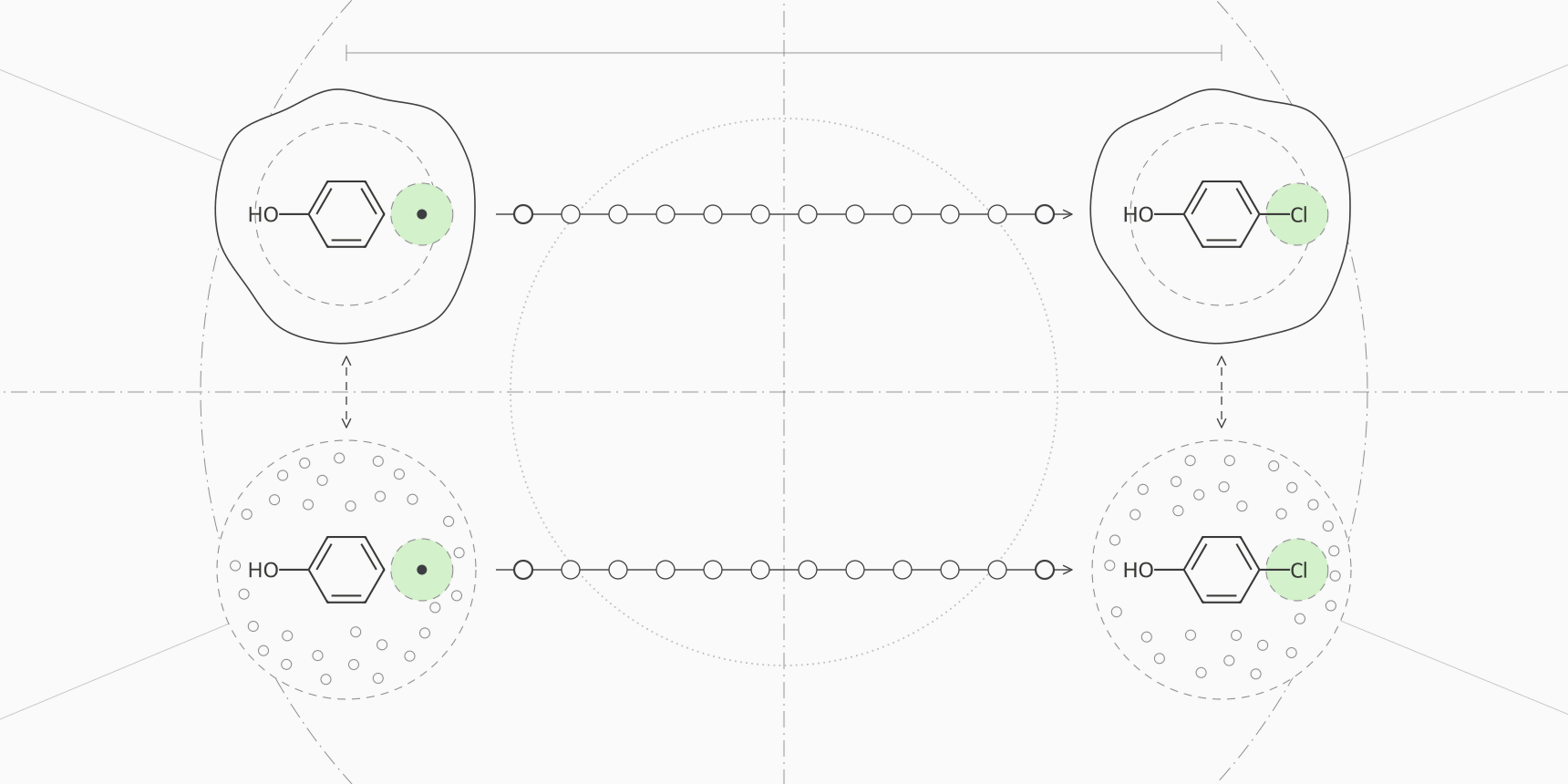
Simulating the binding process directly, with the ligand diffusing out of the pocket into water, would take far longer than any practical simulation. Free energy is a state function, so the path does not matter, and the binding free energy difference between two ligands can be computed around a cycle instead.

The four corners are ligand A bound, ligand B bound, ligand A in water and ligand B in water. The vertical sides are the physical binding events nobody simulates. The horizontal sides are alchemical: mutate A into B inside the protein (the complex leg), and mutate A into B in a box of water (the solvent leg). Because the cycle closes,

$\Delta\Delta G_{\text{bind}} = \Delta G_{\text{bind}}(B) - \Delta G_{\text{bind}}(A) = \Delta G_{\text{complex}}(A \to B) - \Delta G_{\text{solvent}}(A \to B)$

Each leg is a lambda-window calculation of its own. The solvent leg tells you how much water prefers B over A; the complex leg tells you how much the protein environment does. The difference is how much the protein, compared with water, favors the change.

A worked example

Suppose a team wants to know whether replacing a hydrogen on a phenyl ring with chlorine will improve a lead. The numbers below are illustrative, but the arithmetic is exactly what an FEP report contains.

The complex leg, run in 12 windows, returns $\Delta G_{\text{complex}} = -3.6 \pm 0.2$ kcal/mol: the chlorine fills a hydrophobic pocket. The solvent leg returns $\Delta G_{\text{solvent}} = -2.2 \pm 0.1$ kcal/mol. Then

$\Delta\Delta G_{\text{bind}} = -3.6 - (-2.2) = -1.4 \text{ kcal/mol}$

The statistical errors combine in quadrature to about $\pm 0.2$ kcal/mol. A gain of 1.4 kcal/mol corresponds to $10^{1.4/1.36} \approx 11$ times tighter binding. That number is worth acting on only in light of the method's real error, which is several times larger than the ±0.2 kcal/mol from sampling. The accuracy section below puts that error at about 1 to 1.3 kcal/mol on public benchmarks, and the ranking table shows what that does to a 1.4 kcal/mol prediction.

The same cycle runs over every pair in a series. Tools build a perturbation network, usually a minimal spanning graph with a few extra edges forming closed loops. Around a closed loop the ΔΔG values should sum to zero, and the size of the cycle closure error is a quick internal check of convergence.

Relative and absolute binding free energy

The calculation above is relative binding free energy (RBFE): it never computes the affinity of A or B, only their difference. Relative calculations work well because most of the system, the protein, the shared scaffold and most of the solvent, is identical in both states, and errors in it cancel. The price is that every ligand must connect to another by a modest change. Scaffold hops, ring openings and large size changes need more windows and more care, or cannot be connected at all.

Absolute binding free energy (ABFE) decouples a single ligand from its surroundings: its interactions are switched off in the complex and in water, and the difference is $\Delta G_{\text{bind}}$ itself. Restraints keep the vanishing ligand in the pocket, and an analytical correction removes their contribution. ABFE can compare unrelated chemotypes, which is useful for ranking diverse hits, but it samples a much larger change.

Khalak and colleagues calculated absolute binding free energies for 128 protein-ligand complexes and reached an average unsigned error of 1.2 kcal/mol, at roughly ten times the sampling of the corresponding relative calculations.^[8] On the same ligands, relative calculations were still more accurate for ranking within a series: an average error of 3.6 kJ/mol (0.86 kcal/mol) against 4.5 kJ/mol (1.08 kcal/mol) when the relative values were derived from the absolute ones.^[8]

How accurate is free energy perturbation?

Accuracy figures come in several forms, and mixing them up causes most of the confusion in FEP marketing. Edgewise errors compare only the pairs that were simulated. Pairwise errors compare every pair of ligands in a series, including those connected through other edges, and are usually somewhat larger. MUE is the mean unsigned error and RMSE the root mean square error, which weights outliers more.

Study	Method	Dataset	Reported error
Wang 2015	FEP+	199 ligands, 8 targets, 330 edges	RMSE about 1.1; per-target edgewise MUE 0.75 to 1.16
Gapsys 2020	pmx non-equilibrium, Amber and CHARMM consensus	482 perturbations, 13 datasets	Average unsigned error 0.87, the same as FEP+ on those edges
Ross 2023	FEP+	1,237 ligands, 14 datasets	Pairwise RMSE 1.25, MUE 0.98; edgewise RMSE 1.17
Baumann 2026, public set	OpenFE (FEP+ on the same set)	58 systems	Pairwise RMSE 1.73 (FEP+ 1.20)
Baumann 2026, blinded industry set	OpenFE	37 private systems from pharma partners	Pairwise RMSE 2.44
Khalak 2021	Absolute FEP (pmx)	128 complexes	Average unsigned error 1.2 for ΔG

The ceiling is set by experiment. Ross and colleagues collected compounds measured in more than one assay and found a pairwise RMSE of 0.91 kcal/mol between assays of the same compounds, against 0.23 kcal/mol for repeat measurements within one assay.^[5] Kramer's analysis of public Ki values measured by different labs found a mean difference of 0.44 pKi units, about 0.6 kcal/mol.^[9] A method that reaches 1 kcal/mol is therefore not far from the agreement between two labs.

The gap between the public and blinded rows is the most useful number in the table for a buyer. Public benchmarks have been run many times, and their setups have been tuned. On 37 proprietary systems that no developer had seen, OpenFE's pairwise RMSE was 2.44 kcal/mol, and only two systems came in below 1 kcal/mol.^[6] Real projects sit somewhere between the two, depending on how well the target is understood.

What 1 kcal/mol of error means for ranking

An RMSE is hard to act on. The question a chemist asks is how often the calculation puts two compounds in the right order. If prediction errors for a pair are roughly normal with a standard deviation equal to the pairwise RMSE, the chance of ranking the pair correctly is the normal cumulative probability of the true difference divided by that RMSE. We calculated it for three error levels.

True ΔΔG between the pair	Fold difference in Kd	RMSE 1.25 kcal/mol	RMSE 1.0 kcal/mol	RMSE 0.91 kcal/mol
0.5 kcal/mol	2.3×	66%	69%	71%
1.0 kcal/mol	5.4×	79%	84%	86%
1.36 kcal/mol	10×	86%	91%	93%
2.0 kcal/mol	29×	95%	98%	99%
2.73 kcal/mol	100×	99%	>99%	>99%

FEP is unreliable for analogues within a factor of two or three of each other and dependable for differences of tenfold or more. That is enough to be useful. Most changes a chemist proposes are neutral or harmful, and a method that reliably flags the large improvements and large losses removes most of the wasted syntheses, which is what the IRAK4 enrichment shows.

Cost and runtime

FEP is expensive because every edge needs two legs, each with a dozen or more windows of nanosecond-scale sampling, often repeated three times. In 2015 the FEP+ team reported about four perturbations per day on eight GTX 780 GPUs for a system of around 6,000 protein atoms, which works out to roughly 48 GPU-hours per edge on that hardware.^[1] GPUs and protocols have since improved.

The OpenFE industrial benchmark gives a current figure: an average of 5.8 ± 3.4 hours per neutral edge and 31.0 ± 11.3 hours per charge-changing edge on an NVIDIA L40S.^[6] A series of 20 ligands connected by a network with a few redundant loops has around 25 to 30 edges. At the reported per-edge times, an all-neutral network is about 145 to 175 GPU-hours, before setup, failed edges and reruns. One charged analogue connected by two edges adds about 60 more.

Compute is not the main cost. Preparing the protein, assigning protonation and tautomer states, choosing a binding mode, checking that a known reference series reproduces experiment, and reading convergence plots take a computational chemist's time, and that is why outsourced FEP is priced as a project rather than per compound.

Where FEP fails

Every one of these failure modes comes from the same root: the simulation has to sample the states that matter, with a force field that describes them correctly.

Net charge changes are the classic difficulty. Changing a ligand's charge alters long-range electrostatics in a periodic box, and correcting for it needs extra schemes and longer sampling. Chen and colleagues reached an RMSE of 1.1 kcal/mol on 31 charge-changing perturbations with a co-alchemical ion approach.^[10] In the OpenFE benchmark, charge-changing edges were still worse than neutral ones for both codes: an RMSE of 1.65 against 1.29 kcal/mol for OpenFE, and 1.39 against 0.98 for FEP+.^[6]

Scaffold hops and ring changes break the assumption that the two ligands share most of their atoms. Growing or opening a ring passes through strained intermediates that converge slowly. Protocols handle them with softcore potentials and more windows, and they can be modeled accurately, but they cost more and fail more often than R-group changes.^[11][5]

Protonation and tautomer states are fixed at the start of a standard calculation. If the ligand or a binding-site residue changes state on binding, and the simulation uses the wrong one, the answer is wrong however long it runs. The same applies to the binding mode: if analogue B flips in the pocket and the simulation starts it in A's orientation, FEP sees a penalty that does not exist.

Slow motions are the last limit. Buried water molecules that must leave the pocket, side chains that switch rotamer, and loops that rearrange on binding can take longer than the few nanoseconds per window to sample. Repeats that disagree, large cycle closure errors and poor overlap between neighboring windows are the symptoms.

FEP vs docking vs MM/GBSA

The most direct comparison is on the same data. On Wang's eight targets, FEP correlated with experiment at a weighted R of 0.75, MM-GB/SA at 0.35 and Glide SP docking scores at 0.29, and MM-GB/SA was anticorrelated for two of the series.^[1] On a broader benchmark of 285 complexes, AutoDock Vina scores correlated with measured affinity at R = 0.60.^[14] A large 2006 assessment of ten docking programs concluded that none made a useful prediction of binding affinity.^[13]

End-point MM/PBSA and MM/GBSA sit between the two. Genheden and Ryde describe them as often better than docking but worse than FEP, with correlations that range from nothing to excellent depending on the protein, and they warn that rankings are unreliable when affinities differ by less than about 2.9 kcal/mol.^[12] Hou's benchmark found MM/GBSA ranked ligands better than MM/PBSA for most of the six proteins tested.^[15]

	Docking score	MM/GBSA or MM/PBSA	Relative FEP	Absolute FEP
Answers	Does it fit, and roughly how well?	How do these poses compare after MD?	How much does this change help?	How tightly does this ligand bind?
Ligand set	Libraries of thousands to billions	Tens to hundreds of poses	Congeneric series around a known binding mode	Diverse hits with a known pocket
Compute per ligand	Seconds to minutes	An MD run plus minutes of scoring	About 6 GPU-hours per neutral edge on an L40S	About ten times a relative calculation
Typical accuracy	R about 0.6 against affinity	r 0 to 0.9 by protein; unreliable below about 2.9 kcal/mol	RMSE 1.0 to 1.3 kcal/mol on public sets, higher on blinded ones	Unsigned error about 1.2 kcal/mol
Use it to	Find binders and poses	Rescore and remove clear failures; decompose by residue	Choose which analogues to synthesize	Rank chemotypes RBFE cannot connect

In a typical project the methods form a funnel rather than a choice. Docking with AutoDock Vina or GNINA finds poses for a library, a short simulation removes poses that fall apart, MM/GBSA rescoring drops the obvious losers and shows which residues matter, and FEP is reserved for the analogues chemists will actually consider making. Skipping a stage is fine when its question is already answered, for example when a crystal structure fixes the binding mode.

FEP software

Schrödinger's FEP+ is the commercial reference and the method behind most published industrial results. OpenFE, from the Open Free Energy consortium, is the main open-source toolkit, built on OpenMM and the OpenFF force fields, and it is the code the 15-company benchmark tested.^[6] The pmx package runs non-equilibrium alchemical transformations in GROMACS, and Cresset and several academic groups offer their own implementations.

The protocol matters as much as the code. The FEP+ results in the OpenFE benchmark were tuned by hand and run with 20 ns windows, while OpenFE used its standard protocol with 5 ns windows for neutral edges, which likely explains part of the gap between them on the public set.^[6] Any package needs a reference series with known affinities on the target before its predictions are trusted.

Free energy tools on ProteinIQ

ProteinIQ runs the parts of a binding free energy workflow that do not need a hand-tuned FEP setup. The binding free energy calculation use case walks through them in order.

End-point binding free energy:

• gmx_MMPBSA for MM/GBSA and MM/PBSA binding free energies from a GROMACS trajectory, with per-residue decomposition

Alchemical free energy:

• OpenFE for the absolute hydration free energy of a neutral small molecule, a check of the force field and charges for a ligand series; it does not run protein-ligand binding free energies

Simulation and preparation:

• GROMACS for protein and prepared protein-ligand molecular dynamics
• OpenMM for protein simulations with a positioned ligand and OpenFF parameters
• Dimorphite-DL for enumerating ligand protonation states before parameterization

Poses and fast affinity estimates:

• AutoDock Vina and GNINA for docking the starting poses
• Boltz-2 for a predicted complex and affinity value without simulation

Frequently asked questions

What is the difference between FEP and thermodynamic integration?

Both move a system along the same alchemical $\lambda$ path. FEP estimates free energy differences between neighboring windows from energy differences, usually with BAR or MBAR. Thermodynamic integration samples the derivative $\partial U / \partial \lambda$ at each window and integrates it numerically. With enough windows and sampling they give the same answer, and many packages can report both.

How many lambda windows does an FEP calculation need?

Enough that neighboring windows overlap. Published protocols use 11 or 12 windows for neutral R-group changes and up to 16 to 24 for scaffold hops and charge changes.^[5][6] Check the overlap matrix after the run instead of trusting a fixed number: elements next to the diagonal near zero mean a gap the estimator cannot bridge.

Can FEP predict absolute binding affinity?

Absolute FEP can, with an average unsigned error of about 1.2 kcal/mol in the largest published study, but it costs about ten times more than a relative calculation and is more sensitive to the protein structure used.^[8] Relative FEP only gives differences; to turn them into affinities you anchor the series to one compound with a measured value.

Is FEP better than MM/GBSA?

For ranking close analogues, yes. On the same eight targets, FEP correlated with experiment at R = 0.75 against 0.35 for MM-GB/SA.^[1] MM/GBSA is far cheaper, gives per-residue contributions, and is good enough to remove clear failures from a large set of poses, so the two are usually used at different stages.

How long does an FEP calculation take?

On current GPUs, a few hours per neutral edge and about a day or more per charge-changing edge; OpenFE averaged 5.8 and 31.0 hours on an L40S.^[6] By that arithmetic, a neutral series of 20 ligands needs roughly a day on eight GPUs, plus the setup and analysis time, which is usually longer.

Why does my FEP result disagree with experiment?

Check the inputs before the sampling: binding mode, protonation and tautomer states of the ligand and nearby residues, and conserved waters. Then check convergence: disagreement between repeats, cycle closure errors and gaps in window overlap. And compare against the experimental noise; two assays of the same compounds disagree by about 0.9 kcal/mol.^[5]