MM/PBSA vs MM/GBSA: how end-point binding free energies work

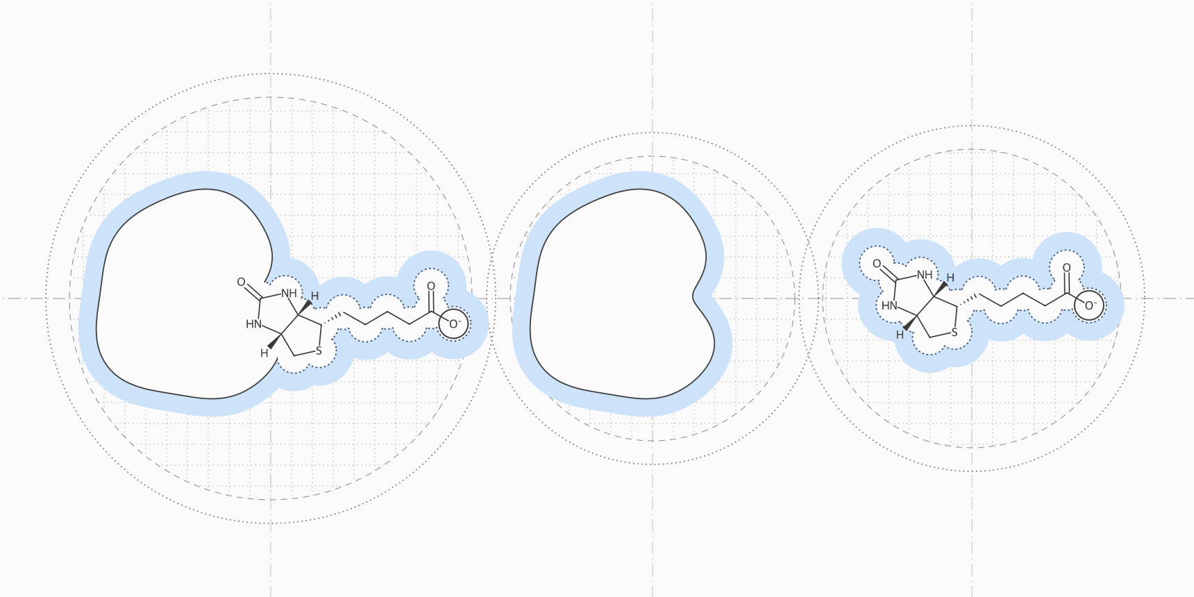
Take a biotin analogue with a negative charge binding to avidin, one of the most studied test systems for binding free energy methods. In an MM/PBSA calculation, the electrostatic attraction between ligand and protein comes out at about −293 kcal/mol. The cost of pulling the ligand's charges out of water, the polar solvation term, comes out at about +293 kcal/mol. The two cancel almost exactly, and the binding free energy is what is left over from van der Waals contacts and smaller terms.^[1]

That cancellation explains most of what goes right and wrong with MM/PBSA and MM/GBSA. Both estimate a binding free energy from snapshots of a molecular dynamics trajectory, and they differ in one term: MM/PBSA gets polar solvation by solving the Poisson-Boltzmann equation numerically, while MM/GBSA approximates it with the analytical generalized Born model.

Because the answer is a small remainder of large opposing terms, the solvation model, dielectric constant and sampling can move it by more than the differences between ligands. In benchmarks, MM/GBSA ranks related ligands about as well as MM/PBSA or better, at a fraction of the cost, and MM/PBSA lands somewhat closer on absolute values.^[3][4] Neither gives an absolute binding free energy you can convert into a Kd. gmx_MMPBSA runs both methods on a GROMACS trajectory.

The end-point idea

The binding free energy is the free energy difference between the complex and the separated receptor and ligand. Alchemical methods such as free energy perturbation (FEP) reach it by gradually transforming one state into another through unphysical intermediates. MM/PBSA, developed by Peter Kollman's group in the late 1990s, samples only the end states and estimates each free energy directly:^[1][2]

$$\Delta G_{\text{bind}} = \langle G_{\text{complex}} \rangle - \langle G_{\text{receptor}} \rangle - \langle G_{\text{ligand}} \rangle$$

The angle brackets are averages over snapshots from molecular dynamics, usually run in explicit water that is stripped out before the energies are calculated. Each free energy is split into the same pieces, so the binding free energy becomes a sum of differences:^[3]

$$\begin{aligned} \Delta G_{\text{bind}} &= \Delta E_{\text{MM}} + \Delta G_{\text{solv}} - T\Delta S \\[4pt] \Delta E_{\text{MM}} &= \Delta E_{\text{internal}} + \Delta E_{\text{elec}} + \Delta E_{\text{vdW}} \\[4pt] \Delta G_{\text{solv}} &= \Delta G_{\text{polar}} + \Delta G_{\text{nonpolar}} \end{aligned}$$

$\Delta E_{\text{MM}}$ is the gas-phase force field energy: bond, angle and dihedral terms, Coulomb electrostatics and Lennard-Jones van der Waals. $\Delta G_{\text{polar}}$ is the electrostatic energy of moving each molecule from vacuum into a dielectric continuum that stands in for water, and it is the term where PB and GB differ. $\Delta G_{\text{nonpolar}}$ covers cavity formation and solute-solvent dispersion, and most implementations estimate it from the change in solvent-accessible surface area:^[1]

$$\Delta G_{\text{nonpolar}} = \gamma \, \Delta\text{SASA} + b$$

Published surface tensions $\gamma$ range from about 0.0024 to 0.057 kcal/mol/Ų, with offsets $b$ from 0 to 1 kcal/mol.^[1] The last term, $-T\Delta S$, is the change in solute entropy, covered in its own section below.

Term	How it is calculated	Avidin example	Typical behavior
ΔE_elec	Coulomb sum over force field charges	−293 kcal/mol	Large and favorable for polar or charged ligands
ΔG_polar	PB or GB continuum electrostatics	+293 kcal/mol	Large and unfavorable; nearly cancels ΔE_elec
ΔE_vdW	Lennard-Jones sum over force field parameters	−35 kcal/mol	Often the term that decides the net result
ΔG_nonpolar	Linear in buried surface area	−4 kcal/mol	Small and similar across related ligands
−TΔS	Normal modes, quasi-harmonic analysis or interaction entropy	Not shown	Unfavorable to binding and the noisiest term; often omitted

Poisson-Boltzmann or generalized Born

Both models treat the solute as a low-dielectric cavity holding fixed atomic charges, surrounded by a high-dielectric solvent, usually with $\varepsilon = 80$ for water. The polar solvation energy is the work of switching that solvent on around the charges. The two models answer the same question with different amounts of approximation.

Poisson-Boltzmann (PB) solves for the electrostatic potential $\phi$ in and around the molecule, given the charge density $\rho$, a dielectric constant $\varepsilon(\mathbf{r})$ that changes at the molecular surface, and mobile ions that screen the field. In its linearized form:^[5]

$$\nabla \cdot \left[\varepsilon(\mathbf{r})\, \nabla \phi(\mathbf{r})\right] - \bar{\kappa}^2(\mathbf{r})\, \phi(\mathbf{r}) = -4\pi\rho(\mathbf{r})$$

Here $\bar{\kappa}$ carries the salt concentration. Programs solve the equation by finite differences on a grid, which makes PB the reference treatment of continuum electrostatics but also slower, and sensitive to grid spacing and to the atomic radii that place the dielectric boundary.^[1][3]

Generalized Born (GB), introduced by Still and colleagues in 1990, replaces the grid with a closed-form sum over pairs of atoms:^[8]

$$\begin{aligned} \Delta G_{\text{polar}} &\approx -\frac{1}{2}\left(\frac{1}{\varepsilon_{\text{in}}} - \frac{1}{\varepsilon_{\text{out}}}\right) \sum_{i,j} \frac{q_i q_j}{f_{\text{GB}}(r_{ij})} \\[4pt] f_{\text{GB}} &= \sqrt{r_{ij}^2 + R_i R_j \exp\!\left(-\frac{r_{ij}^2}{4 R_i R_j}\right)} \end{aligned}$$

$R_i$ is the effective Born radius of atom $i$, a measure of how deeply it is buried in the solute. GB models differ mainly in how they estimate these radii, which is why they give different answers for the same snapshot. Because the energy is a sum over pairs, it splits naturally into per-residue contributions, one reason GB is the usual choice for energy decomposition.^[1]

In AMBER's MMPBSA.py and in gmx_MMPBSA, the GB variant is set with the igb keyword: igb=1 is the model of Hawkins, Cramer and Truhlar, igb=2 and igb=5 are the two parameter sets of Onufriev, Bashford and Case (OBC), and igb=7 and igb=8 are GBn and GBn2.^[11][16]

OBC was built so that GB no longer overstabilizes compact structures relative to PB.^[6] GBn2 refit the GBn parameters on larger data sets and reproduces PB solvation energies of peptides and proteins better than OBC.^[7] In the benchmark by Hou and colleagues, an OBC model ranked ligands best of the three GB models tested.^[3]

How much the choice matters

For seven biotin analogues on avidin, Genheden and Ryde changed only the solvation model and kept everything else fixed. Absolute binding free energies moved by up to 50 kcal/mol between methods, relative values by up to 20 kcal/mol, and the correlation with experiment ranged from 0.59 to 0.93.^[1]

Larger benchmarks give a consistent picture. Hou and colleagues compared PB with three GB models on 59 ligands across six proteins. MM/PBSA was closer on absolute values, but MM/GBSA ranked ligands better for most of the systems without a metal ion in the pocket. Even so, MM/GBSA's mean unsigned error ranged from 4.4 to 21.3 kcal/mol per protein.^[3]

Sun and colleagues then ran both methods on 1,864 complexes from PDBbind. Across the whole set, MM/GBSA correlated better with experiment, with Pearson r of 0.58 against 0.49 for MM/PBSA. Averaged over protein families, which stops a few overrepresented families from dominating, the two were level at about 0.51, and individual families ranged from 0 to 0.9.^[4]

	MM/PBSA	MM/GBSA
Polar solvation	Numerical solution of the PB equation on a grid	Analytical pairwise GB approximation
Speed	Slower	Faster
Per-residue decomposition	Possible, less direct	Natural, because the energy is a pair sum
Main sensitivities	Atomic radii, grid spacing, interior dielectric	GB variant and its radii, interior dielectric
Absolute values	Closer to experiment in Hou et al.	Larger errors in Hou et al.
Ranking ligands	Similar at the protein family level in Sun et al.	Better for most metal-free systems in Hou et al.; r = 0.58 vs 0.49 on all of PDBbind
Needs MD sampling	Yes: r rose from 0.41 on minimized structures to 0.49 with 1 ns of MD	Less: r was 0.58 on minimized structures and 0.56 with 1 ns of MD

One trajectory or three

The first equation asks for three ensembles: the complex, the free receptor and the free ligand. Simulating all three is the three-trajectory protocol. Far more common is the single-trajectory protocol, which simulates only the complex and makes the receptor and ligand snapshots by deleting atoms from each frame:^[1]

$$\Delta G_{\text{bind}} \approx \left\langle G_{\text{complex}} - G_{\text{receptor}} - G_{\text{ligand}} \right\rangle_{\text{complex}}$$

With one trajectory, $\Delta E_{\text{internal}}$ cancels exactly, because the ligand and receptor have the same geometry in both terms, and much of the noise goes with it. The price is that the calculation ignores any change in shape on binding, such as strain in the ligand or a pocket that opens.^[1][3]

The three-trajectory protocol keeps that physics but pays for it in precision. Genheden and Ryde found its standard error four to five times larger, and for ferritin an uncertainty of about 5 kcal/mol made the results practically useless. In practice the single-trajectory protocol often gives the more accurate answer. A middle option also simulates the free ligand, to capture its reorganization energy.^[1]

Precision is a problem even with one trajectory. In early avidin calculations with 20 snapshots, the binding energy fluctuated from frame to frame with a standard deviation of about 11 kcal/mol, leaving a standard error near 3 kcal/mol.^[1] Several short independent simulations beat one long one, because a single long run underestimates its own uncertainty. For avidin, Genheden and Ryde needed 5 to 50 independent runs of 200 ps per ligand to reach a precision of 1 kJ/mol, about 0.24 kcal/mol.^[9]

Longer is not automatically better. Hou and colleagues found that 4.8 ns trajectories gave worse correlations with experiment than 400 ps ones for four of their six proteins, and that 100 snapshots gave the same correlation as 600 taken from the same run.^[3]

The entropy term

$-T\Delta S$ accounts for the freedom that ligand and protein lose on binding: translation, rotation and vibration. It is the hardest term to compute and the one most often left out.^[1] MMPBSA.py offers normal-mode and quasi-harmonic entropy, and gmx_MMPBSA adds interaction entropy and the related C2 entropy; all of them are off by default.^[11][12][16]

Normal-mode analysis is the original method. Each snapshot, trimmed to the residues within roughly 8 to 12 Å of the ligand, is minimized, its vibrational frequencies are calculated, and they are turned into entropies with the harmonic oscillator approximation. It dominates the cost of the whole calculation, is the largest source of statistical noise, and sees only the stiffness of one conformation, not how many conformations are lost on binding.^[1]

Quasi-harmonic analysis builds effective vibrations from the atomic fluctuations along the trajectory. It captures some conformational entropy, but needs very long simulations to converge.^[1]

Interaction entropy, proposed by Duan, Liu and Zhang in 2016, takes the entropy from the fluctuations of the protein-ligand interaction energy that the trajectory already contains, so it adds no extra calculation:^[10]

$$-T\Delta S = kT \ln \left\langle e^{\beta\, \Delta E_{\text{int}}} \right\rangle, \qquad \Delta E_{\text{int}} = E_{\text{int}} - \langle E_{\text{int}} \rangle, \qquad \beta = \frac{1}{kT}$$

Most published MM/PBSA studies leave the entropy out. It is expensive and noisy, and in large tests including it rarely improves the ranking of ligands.^[1] Hou's benchmark is typical: normal-mode entropy clearly improved the correlation for two of six proteins, slightly for one, and not at all for the other three.^[3]

Leaving it out has a cost, though. Binding always costs translational and rotational entropy, so a calculation without the term cannot produce a meaningful absolute free energy.^[1][3]

What the numbers mean

MM/PBSA and MM/GBSA energies are usually too large. In the avidin calculation above, the three charged biotin analogues came out between −35 and −53 kcal/mol, while measured binding free energies for seven avidin ligands reach −20.4 kcal/mol at most.^[1][3] At 25 °C, the conversion from Kd to binding free energy, $\Delta G = RT \ln K_d$, puts even a 1 nM binder at −12.3 kcal/mol, so a calculated value far below that is the method's scale, not a femtomolar affinity.

Because the methods exaggerate differences between ligands, they often achieve a good correlation with experiment and a poor absolute error at the same time, sometimes worse than predicting the same affinity for every ligand.^[1] Read the output as a ranking of related ligands on one target with one protocol, and compare differences against their standard errors. Genheden and Ryde put the practical resolution near 3 kcal/mol: rankings of ligands closer than that are often wrong.^[1]

Some ligand sets break the ranking. Hou and colleagues found good predictions for congeneric series and variable ones for structurally diverse ligands.^[3] Net charge is the classic failure: on PDBbind, the correlation fell from 0.62 for neutral ligands to 0.13 for ligands with a formal charge of 5.^[4]

Interior dielectric constant

The interior dielectric constant $\varepsilon_{\text{in}}$ is the setting that moves results most. Kollman's original formulation used 1. Raising it to 2 or 4 shrinks the electrostatic and polar terms, a crude stand-in for polarization and relaxation of the protein around the ligand.^[1] In Hou's benchmark, avidin's correlation with experiment was 0.92 at $\varepsilon_{\text{in}} = 1$, 0.67 at 2 and 0.51 at 4.^[3]

Hou and colleagues suggested 1 for hydrophobic pockets, 2 for moderately charged ones and 4 for highly charged interfaces with ion pairs to the ligand.^[3] Genheden and Ryde found optimal values anywhere from 1 to 25 depending on the protein and solvation model, with 2 to 4 most often best in studies of several proteins.^[1]

The dielectric constant, the GB variant, whether to include entropy and whether to use MD or minimized structures have all become knobs that can be tuned against experimental data.^[1] A good correlation on a handful of ligands can say more about that tuning than about the method. Fix the protocol before looking at the results, and report the statistical uncertainty with every number.

MM/GBSA compared with docking scores and FEP

Genheden and Ryde summarize where the methods sit: usually more accurate than docking and scoring, less accurate than alchemical methods, with correlations to experiment of about 0 to 0.9 depending on the protein.^[1]

A docking score such as the Vina score evaluates a fitted function on one pose in a rigid receptor, fast enough to rank millions of compounds. AutoDock Vina scores correlated with measured affinity at R = 0.60 on the CASF-2016 benchmark.^[15]

Rescoring docked poses with MM/GBSA adds solvation and explicit electrostatics, and has been used to improve docking and virtual screening results.^[1] Sun's PDBbind results suggest MM/GBSA on minimized poses is a reasonable rescoring step, since it did as well there as with MD.^[4]

Free energy perturbation and related alchemical methods transform one ligand into another through intermediate states, with explicit water throughout. They need much more simulation per ligand pair and work best within a congeneric series, but they are the most accurate physics-based route to relative affinities. Schrödinger's FEP+ protocol was first validated retrospectively on 200 ligands and then used in prospective projects.^[13]

On a later benchmark of 1,237 ligands, Ross and colleagues found FEP+ predicted relative binding free energies with a pairwise RMSE of 1.25 kcal/mol. The same compound series measured in two different assays disagreed by a pairwise RMSE of 0.91 kcal/mol, which sets the floor any method can reach.^[14]

FEP is not always the more expensive choice. For nine factor Xa inhibitors, Genheden and Ryde found an optimized alchemical protocol more efficient than MM/PBSA, because MM/PBSA needed so many independent simulations to become precise.^[1] OpenFE is an open-source alchemical toolkit; on ProteinIQ it runs absolute hydration free energies, a common first check of a ligand's force field and free energy setup before binding calculations.

	Docking score	MM/GBSA or MM/PBSA	FEP
Sampling	One pose, rigid receptor	MD snapshots of the complex	MD along an alchemical path between ligands
Solvent	Implicit in empirical terms	Continuum PB or GB	Explicit water
Ligand sets	Any, including diverse libraries	Best within a series; less sensitive to scaffold changes than FEP	Congeneric series with small changes
Output	Score in kcal/mol units	Estimated ΔG, too large in magnitude	Relative ΔΔG between ligands
Reported accuracy	R = 0.60 for Vina on CASF-2016	r about 0 to 0.9 depending on the protein	Pairwise RMSE 1.25 kcal/mol for FEP+ on 1,237 ligands

Machine learning offers a fourth route. Boltz-2 predicts the complex and an affinity value, a log IC50, from sequence and ligand without any simulation, which places it closer to docking in cost.

Running MM/GBSA on ProteinIQ

A typical end-point calculation starts from a pose, simulates it, and scores the frames.

1. Get a complex. Use a crystal structure, or dock the ligand with AutoDock Vina and check the pose.
2. Simulate the complex in explicit water with GROMACS. OpenMM also runs protein MD, but gmx_MMPBSA reads GROMACS structure, index and trajectory files directly. The protein molecular dynamics use case covers setting up the run.
3. Score the frames with gmx_MMPBSA. Start with MM/GBSA, which is faster and ranks at least as well; run both methods if you want to see how much the solvation model matters for your system. A custom input file sets anything the form does not, such as the interior dielectric or an entropy method.
4. Repeat steps 2 and 3 with independent simulations and compare ligands by the mean and standard error across runs, not by one trajectory.
5. Turn on per-residue decomposition to see which residues drive binding, and treat the totals as a ranking within the series.

The molecular dynamics simulation use case compares the simulation methods and tools available.

Frequently asked questions

Is MM/GBSA more accurate than MM/PBSA?

For ranking related ligands, usually as accurate or better. Hou and colleagues found MM/GBSA ranked ligands better than MM/PBSA for most proteins without metal ions in the pocket, and on PDBbind it correlated better overall and equally well per protein family.^[3][4] MM/PBSA was closer on absolute values in Hou's benchmark, but neither method gives reliable absolute free energies.

Which GB model should I use?

The OBC models (igb=2 or igb=5) and GBn2 (igb=8) are the common choices. GBn2 reproduces PB solvation energies of proteins better, and an OBC model ranked ligands best in Hou's comparison of three GB models.^[7][3] Pick one, keep it for the whole series, and do not compare energies across models.

Why is my MM/GBSA binding energy −50 kcal/mol?

MM/PBSA and MM/GBSA energies are typically much larger in magnitude than measured binding free energies, especially when the entropy term is omitted.^[1] The value is meaningful only relative to other ligands calculated the same way.

Should I include the entropy term?

For ranking similar ligands, it rarely helps and adds a lot of noise and cost.^[1][3] If you need an absolute estimate, or your ligands differ a lot in size and flexibility, include it with enough snapshots for it to converge; interaction entropy costs nothing extra on top of the MD.^[10]

How long should the MD simulation be?

Several independent short runs are better than one long one. Genheden and Ryde recommend about 100 ps of equilibration and 20 to 200 ps of production per run, repeated until the standard error is small enough for the comparison you want to make.^[9]

When should I use FEP instead?

When you need to separate close analogues in lead optimization and can afford the simulation. MM/GBSA rankings of ligands closer than about 3 kcal/mol are unreliable, while FEP is built for small changes within a series.^[1][14]