SASA calculator
Calculate solvent accessible surface area for protein structures
Input
Output
Configure input settings on the left, then click "Calculate"
Calculate solvent accessible surface area for protein structures
Assign protein secondary structure using the DSSP algorithm. The gold standard for hydrogen bond-based structure assignment from coordinates.
Validate protein structure quality with all-atom contact analysis, Ramachandran plots, rotamer assessment, and geometry checks.
Generate a downloadable PDBsum structural summary report archive for a single protein structure.
Calculate the radius of gyration (Rg) for protein structures from PDB files. Supports multiple chains and atom selection options.
Calculate Root Mean Square Deviation (RMSD) between protein structures. Compare a reference PDB against multiple structures with automatic Kabsch alignment.
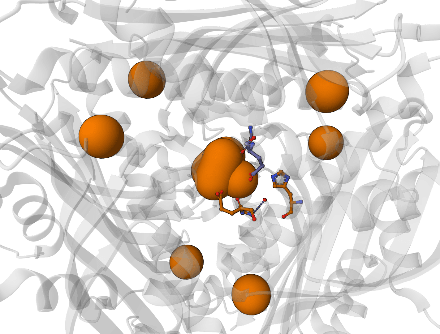
Predict metal and water binding sites in protein structures using 3D convolutional neural networks (AllMetal3D + Water3D).
Assess docking model quality by comparing predicted complexes against native references. DockQ v2.1.3 supports protein, nucleic-acid, and supported small-molecule interfaces with faithful native metrics.
Scoring function for interprotein interactions in AlphaFold2, AlphaFold3 and Boltz predictions. Calculates ipSAE, ipTM, pDockQ, pDockQ2, and LIS scores to assess protein-protein interface quality.
PoseBusters validates generated or docked molecular poses with chemically and structurally grounded quality checks for molecular geometry, intermolecular interactions, and optional reference-pose agreement.
Geometric deep learning model for predicting protein binding sites directly from 3D structure. Identifies where proteins interact with other proteins, antibodies, or disordered proteins with high accuracy, including for novel protein folds.
Solvent Accessible Surface Area (SASA) measures how much of a protein's surface is exposed to the surrounding solvent. This property reveals which residues are on the protein's exterior versus buried in its hydrophobic core.
SASA is fundamental to understanding protein folding, stability, and function. Exposed hydrophobic residues often indicate binding sites or regions that may aggregate. Changes in SASA between conformational states can quantify domain movements or ligand-induced structural changes.
For a comprehensive analysis of your structure, combine SASA with other structural tools like the Ramachandran Plot for backbone geometry or DSSP for secondary structure assignment.
The Shrake-Rupley algorithm calculates SASA by computationally "rolling" a probe sphere (representing a water molecule) over the protein surface. First introduced in 1973, it remains the standard method for SASA calculation.
Each atom is represented as a sphere with its van der Waals radius. The algorithm expands these radii by the probe radius (typically 1.4 Å for water) to create an accessible sphere. Points distributed on this expanded sphere are tested for overlap with neighboring atoms.
The accessible surface area for each atom equals the fraction of test points not buried by neighbors, multiplied by the sphere's surface area:
where is the van der Waals radius plus the probe radius, and is the number of test points.
The algorithm uses standard van der Waals radii for each element. Carbon atoms have a radius of 1.7 Å, nitrogen 1.55 Å, oxygen 1.52 Å, and sulfur 1.8 Å. These radii define the physical size of each atom.
For residue-level output, the calculator also reports relative accessibility—the percentage of a residue's surface that is exposed compared to its maximum possible exposure. This is calculated as:
Maximum SASA values are derived from Gly-X-Gly tripeptides, representing a fully exposed residue. Residues with relative accessibility below 20% are typically considered buried, while those above 50% are surface-exposed.
Upload one or more PDB files containing your protein structure. The calculator processes ATOM records and ignores hydrogen atoms by default. You can also fetch structures directly from the RCSB PDB using their 4-character IDs.
Output level: Choose the granularity of results. Structure returns a single total SASA value. Chain breaks down SASA by each polypeptide chain. Residue provides per-residue accessibility, which is most useful for identifying surface-exposed positions.
Probe radius: The radius of the virtual solvent sphere. The standard value of 1.4 Å represents a water molecule. Larger probes (1.8–2.0 Å) can model bulkier solvents or identify only the most accessible regions.
At the structure level, you get the total SASA in Ų along with counts of chains and residues. Typical globular proteins have SASA values ranging from a few thousand to tens of thousands of Ų, depending on size.
Each chain is listed separately with its total SASA and residue count. This is useful for comparing surface exposure between subunits or identifying which chains contribute most to the complex's surface.
The most detailed view shows:
Residues with high relative accessibility are good candidates for surface mutations or chemical modifications. Those with unexpectedly low accessibility despite being charged (Lys, Arg, Glu, Asp) may indicate buried salt bridges.
SASA analysis is valuable when designing mutations—you can confirm a target residue is surface-exposed before introducing modifications. It also helps identify potential binding interfaces, which often show intermediate accessibility values.
Comparing SASA between apo and ligand-bound structures quantifies the buried surface area upon binding, which correlates with binding affinity. Monitoring SASA changes across molecular dynamics trajectories reveals conformational dynamics.
The Shrake-Rupley algorithm treats the protein as a static structure. For flexibility, consider analyzing multiple conformations from NMR ensembles or molecular dynamics. The calculation excludes hydrogen atoms by default, which slightly underestimates true SASA.
Relative accessibility values assume the Gly-X-Gly reference state, which may not perfectly represent the local environment for all residues. Values exceeding 100% can occur for residues in extended conformations.